a quick video showing how to add new points to an existing point layer using GPS coordinates, and some discussions
access original video site@ http://www.utipu.com/app/tip/id/16335/
Friday, September 11, 2009
Add Points to Existing Layer from Coordinates
a quick video showing how to add new points to an existing point layer using GPS coordinates, and some discussions
access original video site@ http://www.utipu.com/app/tip/id/16335/
access original video site@ http://www.utipu.com/app/tip/id/16335/
Thursday, September 10, 2009
Blog Site Migration
Due to some of the "difficulties" of using Blogspot.com, I'm migrating this blog over to Wordpress.com service.
Please visit http://zliu95618.wordpress.com/ for future posts.
Thanks!
Please visit http://zliu95618.wordpress.com/ for future posts.
Thanks!
Wednesday, September 9, 2009
SWARS Spatial Analysis, The Book (7)
Create The "Perfect" Boundary...
Off we go now!
I start by bringing in all the 7 input layers (provided in the example data pacaket). The seven layers are:
1. WaterIntake (Point)
2. Invasive (Point)
3. Stream (Line)
4. River (Line)
5. Watershed (Polygon)
6. LandCover (Polygon)
7. DEM (Grid)

We have two existing polygon layers here, the Watershed layer and the LandCover layer. When you zoom in to the coast areas, you will see a lot of these "gaps" as pointed out in this image:

Using either of these two polygon layers as the analysis mask, you will end up losing some data. A compromise? I will use the Union tool to merge these two polygon layers together.

(Shown on the image above)
I know which tool I will use already. So, I just go to Arctoolbox, click the <Index>Tab (at the bottom). Then type in the key word "Union" to locate the tool. Double-click on the already highlighted <Union> tool to launch the function.
Just follow the dialog, using Watershed and Landcover as the two Input Features, I will create a output Feature Class (shapefile) named Land_Union.
Once the tool is run, ArcMap will automatically bring in the output layer. Just color it up using a solid green with no border line and here is what you get:

As you can see, all the "gaps" are now closed and covered!
Next, open the attribute table of this newly created Land_Union layer. Create a new attribute field and name it "LandValue" using Short Integer type. And leave the value as t he default "0". If you want to use any other value, just use the <Field Caculator> tool to assign the new integer value.

Close the table.
I will then use the <Zoom>tools to make a nice and snuggy rectangle just around the Babeldabo area which I will use as my Analysis Extent!
Now, open the Spatial Analyst Option dialog again to set the analysis environment. Click on <Spatial Analyst>menu, then in the drop-down list, click <Options>.

Under <General> Tab, I will
* set my Working Directory to where I want to put all the output layers, and
* use Land_Union as the Analysis Mask.
* for Analysis Coordinate System, select the second option and use the active data frame's coordinate system.
(*** the data frame's coordinate system is defined by the first data layer you brought into the frame!!!)
In<Extent> Tab,
* set the Analysis Extent to "Same as Display" (choose from the drop-down list), then
* set the Snap Extent to the DEM layer (dem_nad83).
Finally, under<Cell Size> Tab, |
* set the Analysis Cell Size to "Same as Layer "dem_nad83".
With the Analysis Environment set, we are ready to push forward!!
|
Highlight the Land_Union layer by click on it in the Table of Content (TOC).
Click <Spatial Analyst>again, choose <Convert>, then <Features to Raster...>.
The Features to Raster dialog will now open. If you highlighted the Land_Union layer first, it should be selected as the Input Features already. If you didn't, no worries either. Just select it use the drop-down list.
Choose "LandValue" as the Field from the list.
Output Cell Size should already be 10. |
In the last option, I will name the output raster as Land_Union_R (with the R for "Raster"). Hit OK!
When it's done, we now have our "Perfect Boundary/Background" which is already defined to the most efficient spatial extent (try use the zoom to layer tool and see where it goes), with the right project and cell size, all thanks to the previous setting of the Analysis Environment!! | 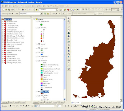
Off we go now!
I start by bringing in all the 7 input layers (provided in the example data pacaket). The seven layers are:
1. WaterIntake (Point)
2. Invasive (Point)
3. Stream (Line)
4. River (Line)
5. Watershed (Polygon)
6. LandCover (Polygon)
7. DEM (Grid)

We have two existing polygon layers here, the Watershed layer and the LandCover layer. When you zoom in to the coast areas, you will see a lot of these "gaps" as pointed out in this image:

Using either of these two polygon layers as the analysis mask, you will end up losing some data. A compromise? I will use the Union tool to merge these two polygon layers together.

(Shown on the image above)
I know which tool I will use already. So, I just go to Arctoolbox, click the <Index>

Next, open the attribute table of this newly created Land_Union layer. Create a new attribute field and name it "LandValue" using Short Integer type. And leave the value as t

I will then use the <Zoom>
Now, open the Spatial Analyst Option dialog again to set the analysis environment. Click on <Spatial Analyst>

* set my Working Directory to where I want to put all the output layers, and
* use Land_Union as the Analysis Mask.
(*** the data frame's coordinate system is defined by the first data layer you brought into the frame!!!)
In
* set the Analysis Extent to "Same as Display" (choose from the drop-down list), then
* set the Snap Extent to the DEM layer (dem_nad83).
Finally, under
* set the Analysis Cell Size to "Same as Layer "dem_nad83".
With the Analysis Environment set, we are ready to push forward!!
Click <Spatial Analyst>
The Features to Raster dialog will now open. If you highlighted the Land_Union layer first, it should be selected as the Input Features already. If you didn't, no worries either. Just select it use the drop-down list.
Choose "LandValue" as the Field from the list.
Output Cell Size should already be 10.
In the last option, I will name the output raster as Land_Union_R (with the R for "Raster"). Hit OK!
When it's done, we now have our "Perfect Boundary/Background" which is already defined to the most efficient spatial extent (try use the zoom to layer tool and see where it goes), with the right project and cell size, all thanks to the previous setting of the Analysis Environment!!

Tuesday, September 8, 2009
SWARS Spatial Analysis, The Book (6)
*Go to ArcGIS Desktop Help, read as much as you can find about Spatial Analyst and Raster Analysis Environment Settings.
Turn on the Spatial Analyst
First thing first! For this SWARS analysis, the most important group of ArcGIS functions is in the Spatial Analyst Extension. So, make sure you even have that extension!
To get the ArcMap Spatial Analyst toolbar out, if you have the extension installed and licensed:
1. in ArcMap, click the
2. select
3. in the Extensions dialog, check on the Spatial Analyst extension
4. then, click the
5. select
6. check the Spatial Analyst option
You should now see the Spatial Analyst toolbar on your main ArcMap interface.
If you don't see the Spatial Analyst option, that means you don't have that extension for your ArcGIS. You will need some extra help getting it solved.
Now, here are a few very important concepts which we will apply but you might not have paid enough attention to before.
* Analysis Mask
* Analysis Extent
* Snap Raster
* Cell Size
Ding! Ding! Ding! Any bell rings?? If not, you should and can find all the explanations you need in ArcGIS Desktop Help. Just go into the Help and type in those key words to find them. I will explain a bit more when we get to them.
Get familiar with these key concepts first. It's worth the time!!
**ArcGIS Desktop Help is your first and perhaps one of the best places to go for information on how to use ArcGIS! Get used to it!
Now you should see the Spatial Analyst toolbar on your main ArcMap interface. Click on
The raster analysis Environment Settings dialog box will appear as shown here.

This is where you do it once and save a whole lot of time later.
As I said during the Hawaii SWARS Workshop, ideally, we would have a boundary polygon (Analysis Mask) that encompasses precisely all and only the areas we will be analyzing, which itself is so well defined within such a "snuggy" rectangle (Analysis Extent)! Should such a national treasure exist, all shall be easy. We can just use it for all our raster analysis environment settings.
Unfortunately, many of us don't score that lottery. Therefore, we are likely required to "create" it! This is where it gets interesting and creativity shall shine.
Case Example
For our Palau exercise, we will:
* limit our Analysis Extent to the Babeldabo island;
o you want the Analysis Extent to be as small as possible;
* snap all rasters to the existing DEM grid; and
o use one of your existing rasters as the snap raster;
* set our output raster cell size to the same as the DEM grid, 10 by 10 meters.
o 10 by 10 feels about right for the size of most of the islands.
Again, it's up to you to determine exactly how to set those parameters!
Thursday, September 3, 2009
Slow down my ranting
The techy part of this BOOK should supposedly be the easiest part for me, because that's what I do. I joked all the time during our workshops, that I can finish a SWARS for pretty much any of the islands in a couple of hours, from start to finishing the metadata. That "joke" wouldn't be too far off from the truth. But, often times, however, explaning what you are good at to a wider audience is a lot more difficult than it looks.
We simply take too much for granted for what we are familiar with. Sometimes, when I ask my firends working in the valley for help, I just have to tell them to slow down. There is nothing embarrasing about that.
12 years of expeirence does make a difference. For 12 years I have been using GIS software, especially the ESRI product. That sometimes makes me think too easily that everybody should just already know something in ArcGIS, which of course is not true. Slowing it down is always good.
To prepare this exercise, I have run the analysis a couple of times already, trying various options and combinations. Remember, I keep emphasizing that there are almost always multiple choices to accomplish a task in ArcGIS and there is often no right or wrong chosing any. So, the procedure I present here is what I think is appropriate and perhaps more importantly, smooth.
Videos will be made available to accompany the document. Nothing is more effective, when it comes to learning how to use a software, than simply watching others do it.
Wednesday, September 2, 2009
Download the Palau SWARS Example Data
If you want to follow exactly how The Book runs through the Palau example analysis, download the data packet here.
SWARS Spatial Analysis, The Book ( Case Example )
Since we are getting into the hands-on dirty techy stuff, we'd need an example to run on. Data provided by our partners from the PALARIS office in Palau will be used. Special thanks to PALARIS!
The Issue
The "ISSUE" for the sample analysis is defined as "protect and improve water quality". When all processes are run, the final priority map will show the important areas where forestry grograms can better help to protect and improve the water quality for Palau and its population.
The Input Layers
These are the six input layers and their weights:
It's pretty straightforward that the Priority Watershed layer is ranked the highest for our case issue. The Land Cover layer is ranked right up there too because it provides an array of critical attributes regarding water quality. It identifies where the critical land cover types are, e.g. wetlands and forests. You can also extract wildfire risk from it. Obviously, the river and stream systems are important (these two usually are combined in one layer). The Invasive species layer reveals an significant aspect of the forest health. It is also used to demonstrate how to use a point source layer. Slope, well, at least it tells you the level of difficulty to operate.
Satisfactory? Maybe not as much as I prefer, but good enough perhaps for the purpose of demonstrating the process.
The RCV Classificationon Scheme
A RCV Scheme of 1 to 10 step by 1.
** Please note!!! The Palau case example used here is only for the purpose of going through the GIS techniques. It is NOT an actual SWARS project. Layers selection is mostly based on data availability. The Invasive Species point data is created by the author and not an actual layer!!
The Issue
The "ISSUE" for the sample analysis is defined as "protect and improve water quality". When all processes are run, the final priority map will show the important areas where forestry grograms can better help to protect and improve the water quality for Palau and its population.
The Input Layers
These are the six input layers and their weights:
- Priority Watershed; (polygon); 25%
- Land Cover Types; (Polygon); 25%
- River; (Line); 15%
- Stream (Line); 15%
- Invasive Species*; (Point); 15%
- Slope; (Grid); 5%
*Unlike the other five, the Invasive Species layer is not an actual dataset but created by the author to demonstrate how can a point layr be used creatively.
Not to be forgotten is an good explanation why these layers are used and used as such. So, here is my "why":It's pretty straightforward that the Priority Watershed layer is ranked the highest for our case issue. The Land Cover layer is ranked right up there too because it provides an array of critical attributes regarding water quality. It identifies where the critical land cover types are, e.g. wetlands and forests. You can also extract wildfire risk from it. Obviously, the river and stream systems are important (these two usually are combined in one layer). The Invasive species layer reveals an significant aspect of the forest health. It is also used to demonstrate how to use a point source layer. Slope, well, at least it tells you the level of difficulty to operate.
Satisfactory? Maybe not as much as I prefer, but good enough perhaps for the purpose of demonstrating the process.
The RCV Classificationon Scheme
A RCV Scheme of 1 to 10 step by 1.
** Please note!!! The Palau case example used here is only for the purpose of going through the GIS techniques. It is NOT an actual SWARS project. Layers selection is mostly based on data availability. The Invasive Species point data is created by the author and not an actual layer!!
Tuesday, September 1, 2009
Island Imagery Available (August 2009)
Let's get away from the boring "book" for a while and take a look at what imagery we have for the islands as of today. Here is an update.
*********************************************************************************
· Latest update
o Kosrae (FSM) Pan-sharpened Natural Color QuickBird; August 2008 from Tony Kimmet (NRCS)
o Kosrae (FSM) Pan-sharpened Color-Infrared QuickBird; August 2008 from Tony Kimmet (NRCS)
o Manu’a group (American Samoa) Pan-sharpened Natural Color QuickBird; August 2008 from Land Info (direct purchase).
o Manu’a group (American Samoa) Pan-sharpened Color-Infrared QuickBird; August 2008 from Land Info (direct purchase).
· All Archive Imagery Available
Island Imagery Available
Guam IKONOS; QuickBird
CNMI IKONOS; QuickBird
Palau QuickBird
American Samoa QuickBird
Federated States of Micronesia QuickBird
Republic of the Marshall Islands QuickBird
Hawaii QuickBird
· Data Distribution Status
o All archive image data have been distributed to corresponding islands/sates with the latest transfer provided as part of our workshop materials.
o The new Manu’a group QuickBird has been provided to American Samoa.
SWARS Spatial Analysis, The Book (5)
Design Raster Class Value Classification Scheme...
OK! By now, you supposedly have defined the issue, chosen the input layers, and assigned the layer weights. It's finally time to get into the GIS thingy!

* The Scream by Edvard Munch, 1893
No, no, no. No need to scream. Take it easy! All will be just fine.
Start the engine...
Your input layers are likely to exist in all kinds of GIS data types, polygon vector, line vector, point vector, or raster grid, etc. But our final model takes only one data type -- Raster Integer Grid. That means, there is a lot of work to be done just to get the input layers ready. For those of you who attended our Hawaii SWARS Workshop, you would probably agree with me that this part of the project -- to get the layers ready -- is perhaps the most "difficult" part for us, the GIS specialists.
We start this long journey with the Raster Class Value (RCV) Classification Scheme.
Whatever type the original data is, we need to "transform" it into an Integer Grid, because that's what the final model requires. A weighted overlay basically is to sum up the weighted values of coincident pixels from all input layers. A pixel is a square unit that represents a specific area on the ground. If we consider each input layer as a factor/element/feature in the overall analysis, a pixel will carry a unique value for each factor (layer) that represents the value of that particular area for that factor (layer).
Note that we actually have two weighting/ranking processes through this project.
First, we rank and assign weights to each input layers based on their relative importance to the analysis.
Then, we rank and assign values to each pixel/area of land within each input layer.
All lands should not be treated as the same because of their locations. Neither should the same land be looked at as the same depending on what you are looking for. A remote wildness area is probably much more attractive if you are searching for natural beauty compared to a downtown center. But the same wildness area is not likely to be your first choice for a new elementary school or shopping center. Simple, right?
The RCV Classification Scheme is applied to the relative value of each pixel within a input layer. Again, all lands should not be treated as the same depending on their location. Say we are looking at the watershed layer. Some watersheds are significantly more important than others because they supply water to the public drinking system. Hence, we are assigning higher values to the land within these priority watersheds. A question presents. What is the value?
Well, I guess that's why we need to establish a RCV Scheme first.
If you have done the Spatial Analysis Project (SAP), you would know already that for SAP, it's a binary value system. So, the pixel value will be either 0 or 1, very simple. In fact, if you want, you could use the same binary value system for SWARS. Some states indeed are doing so. However, that choice would not be my recommendation.
I suggest a wider value range than what you absolutely need. For example, if the maximum number of values you need is 5 (1~5), then use a value systems than provides a range of 10 (1~10). Remember, you do not have to actually use all the values available! But one thing I will remind again, make sure you do use the Maximum value for each layer! You must not unconsciously mixed in a layer ranking here when you are supposed to only rank the land within a layer.
Say if you have a RCV scheme of 1 to 10. For layer A you used values 10, 8, 5, 3, 1. But for layer B, you used 7, 4, 2. In this example, you already have a 10 to 7 weighting ratio against layer B!! Leave that to your layer weights!!
Again, two points to take from the example above. First, you do NOT have to use up all the values available in the RCV scheme. Two, you should/must employ the maximum value in the RCV scheme for each input layer.
Oh, one more thing which I also repeatedly advocated in our Hawaii Workshop, do NOT use the value 0! There are multiple reasons why I say that especially coming from a long history of using software like ERDAS. One reason you will see later on.
Case Example
So, for our case example of Palau, I will use a RCV scheme of 1 to 10 step by 1.
OK! By now, you supposedly have defined the issue, chosen the input layers, and assigned the layer weights. It's finally time to get into the GIS thingy!
* The Scream by Edvard Munch, 1893
No, no, no. No need to scream. Take it easy! All will be just fine.
Start the engine...
Your input layers are likely to exist in all kinds of GIS data types, polygon vector, line vector, point vector, or raster grid, etc. But our final model takes only one data type -- Raster Integer Grid. That means, there is a lot of work to be done just to get the input layers ready. For those of you who attended our Hawaii SWARS Workshop, you would probably agree with me that this part of the project -- to get the layers ready -- is perhaps the most "difficult" part for us, the GIS specialists.
We start this long journey with the Raster Class Value (RCV) Classification Scheme.
Whatever type the original data is, we need to "transform" it into an Integer Grid, because that's what the final model requires. A weighted overlay basically is to sum up the weighted values of coincident pixels from all input layers. A pixel is a square unit that represents a specific area on the ground. If we consider each input layer as a factor/element/feature in the overall analysis, a pixel will carry a unique value for each factor (layer) that represents the value of that particular area for that factor (layer).
Note that we actually have two weighting/ranking processes through this project.
First, we rank and assign weights to each input layers based on their relative importance to the analysis.
Then, we rank and assign values to each pixel/area of land within each input layer.
All lands should not be treated as the same because of their locations. Neither should the same land be looked at as the same depending on what you are looking for. A remote wildness area is probably much more attractive if you are searching for natural beauty compared to a downtown center. But the same wildness area is not likely to be your first choice for a new elementary school or shopping center. Simple, right?
The RCV Classification Scheme is applied to the relative value of each pixel within a input layer. Again, all lands should not be treated as the same depending on their location. Say we are looking at the watershed layer. Some watersheds are significantly more important than others because they supply water to the public drinking system. Hence, we are assigning higher values to the land within these priority watersheds. A question presents. What is the value?
Well, I guess that's why we need to establish a RCV Scheme first.
If you have done the Spatial Analysis Project (SAP), you would know already that for SAP, it's a binary value system. So, the pixel value will be either 0 or 1, very simple. In fact, if you want, you could use the same binary value system for SWARS. Some states indeed are doing so. However, that choice would not be my recommendation.
I suggest a wider value range than what you absolutely need. For example, if the maximum number of values you need is 5 (1~5), then use a value systems than provides a range of 10 (1~10). Remember, you do not have to actually use all the values available! But one thing I will remind again, make sure you do use the Maximum value for each layer! You must not unconsciously mixed in a layer ranking here when you are supposed to only rank the land within a layer.
Say if you have a RCV scheme of 1 to 10. For layer A you used values 10, 8, 5, 3, 1. But for layer B, you used 7, 4, 2. In this example, you already have a 10 to 7 weighting ratio against layer B!! Leave that to your layer weights!!
Again, two points to take from the example above. First, you do NOT have to use up all the values available in the RCV scheme. Two, you should/must employ the maximum value in the RCV scheme for each input layer.
Oh, one more thing which I also repeatedly advocated in our Hawaii Workshop, do NOT use the value 0! There are multiple reasons why I say that especially coming from a long history of using software like ERDAS. One reason you will see later on.
Case Example
So, for our case example of Palau, I will use a RCV scheme of 1 to 10 step by 1.
Subscribe to:
Posts (Atom)


