SWARS Spatial Analysis, The Book (7)

Create The "Perfect" Boundary...

Off we go now!

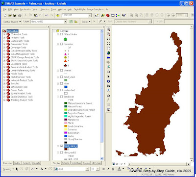
I start by bringing in all the 7 input layers (provided in the example data pacaket). The seven layers are:

1. WaterIntake (Point)
2. Invasive (Point)
3. Stream (Line)
4. River (Line)
5. Watershed (Polygon)
6. LandCover (Polygon)
7. DEM (Grid)



We have two existing polygon layers here, the Watershed layer and the LandCover layer. When you zoom in to the coast areas, you will see a lot of these "gaps" as pointed out in this image:



Using either of these two polygon layers as the analysis mask, you will end up losing some data. A compromise? I will use the Union tool to merge these two polygon layers together.


(Shown on the image above)

I know which tool I will use already. So, I just go to Arctoolbox, click the <Index> Tab (at the bottom). Then type in the key word "Union" to locate the tool. Double-click on the already highlighted <Union> tool to launch the function.

Just follow the dialog, using Watershed and Landcover as the two Input Features, I will create a output Feature Class (shapefile) named Land_Union.

Once the tool is run, ArcMap will automatically bring in the output layer. Just color it up using a solid green with no border line and here is what you get:


As you can see, all the "gaps" are now closed and covered!

Next, open the attribute table of this newly created Land_Union layer. Create a new attribute field and name it "LandValue" using Short Integer type. And leave the value as the default "0". If you want to use any other value, just use the <Field Caculator> tool to assign the new integer value.


Close the table.

I will then use the <Zoom> tools to make a nice and snuggy rectangle just around the Babeldabo area which I will use as my Analysis Extent！


Now, open the Spatial Analyst Option dialog again to set the analysis environment. Click on <Spatial Analyst> menu, then in the drop-down list, click <Options>.


Under <General> Tab, I will

* set my Working Directory to where I want to put all the output layers, and
* use Land_Union as the Analysis Mask.
* for Analysis Coordinate System, select the second option and use the active data frame's coordinate system.
(*** the data frame's coordinate system is defined by the first data layer you brought into the frame!!!)


In <Extent> Tab,

* set the Analysis Extent to "Same as Display" (choose from the drop-down list), then
* set the Snap Extent to the DEM layer (dem_nad83).


Finally, under <Cell Size> Tab,

* set the Analysis Cell Size to "Same as Layer "dem_nad83".


With the Analysis Environment set, we are ready to push forward!!

Highlight the Land_Union layer by click on it in the Table of Content (TOC).

Click <Spatial Analyst> again, choose <Convert>, then <Features to Raster...>.

The Features to Raster dialog will now open. If you highlighted the Land_Union layer first, it should be selected as the Input Features already. If you didn't, no worries either. Just select it use the drop-down list.

Choose "LandValue" as the Field from the list.

Output Cell Size should already be 10.

In the last option, I will name the output raster as Land_Union_R (with the R for "Raster"). Hit OK!

When it's done, we now have our "Perfect Boundary/Background" which is already defined to the most efficient spatial extent (try use the zoom to layer tool and see where it goes), with the right project and cell size, all thanks to the previous setting of the Analysis Environment!!